Usage
To use perfume in a project:
import perfume
# In a Jupyter notebook, you'll want these to get the plots to
# display inline
import bokeh.io
bokeh.io.output_notebook()
Collecting samples
The entry point to perfume is perfume.bench(), which
takes a list of Python functions, and benchmarks them together. It
will display, and update:
A plot showing histograms of sampled latencies for each function, with a kernel density estimator and 25th, 50th, and 75th percentiles.
A table of
pandas.DataFrame.describe()output for the sampled timings.Two pairwise Kolmogorov-Smirnov test tables, one on the raw samples, the other more sensitive to outliers (more on how later).
Analyzing results
When you run perfume.bench(), it returns a
DataFrame of the samples, represented as wall-clock
begin and end times. There are several built-in ways to
interpret these, collected in perfume.analyze, a few examples
here:
perfume.analyze.timings()interprets thebegin/endtimes in the samplesDataFrameand computes the differences betweenendandbegin, giving you a newDataFramecontaining elapsed time values.perfume.analyze.isolate()adjusts each function’sbegin/endtimes to be as if that function was benchmarked in isolation, so eachbeginmatches the previousend. This can be interpreted as “time to simulated completion” of a given fixed-size workload.perfume.analyze.ks_test()runs the Kolmogorov-Smirnov test across the benchmarked functions (given output fromperfume.analyze.timings()), giving pairwise results. The 2-sample K-S test is a measure of how different two distributions are (briefly, it’s the largest vertical distance between their ECDFs). For a function you think you’ve optimized, you can run the old and new versions and use the K-S test to get a sense for how likely it is that you’ve made a consistent improvement.perfume.analyze.cumulative_quantiles_plot()creates a plot over time of the median, upper and lower quantiles, and min and max, for all samples collected up until that point in simulation time. Each function is charted with its timings in isolation (seeperfume.analyze.isolate()), so faster functions cover less of the x-axis. For example: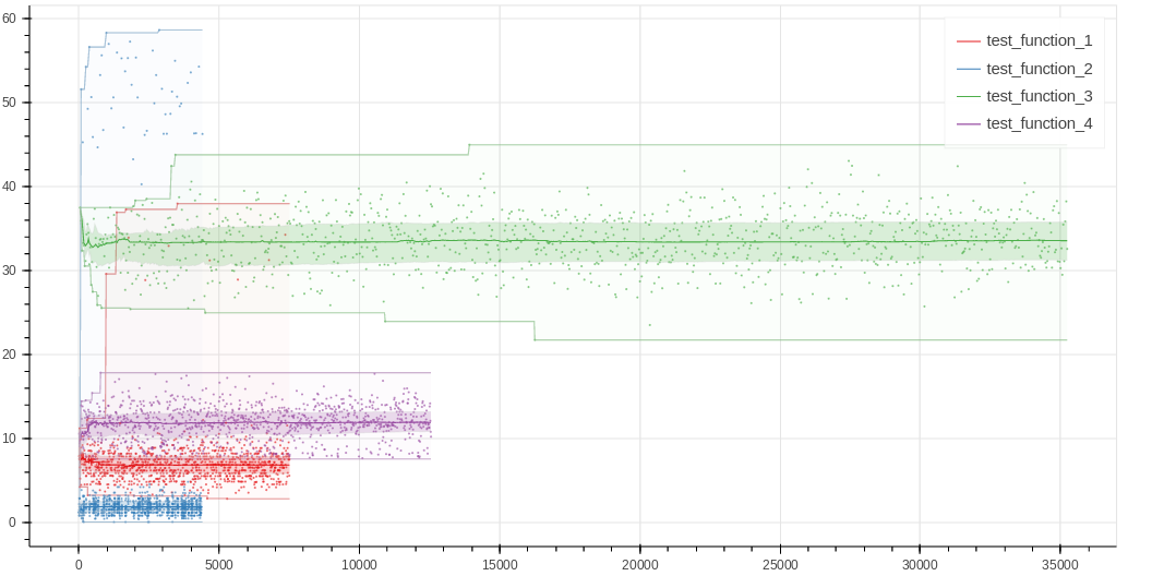
See perfume.analyze for the full set of analysis tools.