Example notebook
[1]:
import perfume
import perfume.analyze
import pandas as pd
import bokeh.io
bokeh.io.output_notebook()
Setup
To start, set up some functions to benchmark.
[2]:
import time
import numpy as np

def test_fn_1():
    good = np.random.poisson(20)
    bad = np.random.poisson(100)
    msec = np.random.choice([good, bad], p=[.99, .01])
    time.sleep(msec / 3000.)

def test_fn_1_no_outliers():
    time.sleep(np.random.poisson(20) / 3000.)

def test_fn_2():
    good = np.random.poisson(5)
    bad = np.random.poisson(150)
    msec = np.random.choice([good, bad], p=[.95, .05])
    time.sleep(msec / 3000.)

def test_fn_3():
    msec = max(1, np.random.normal(100, 10))
    time.sleep(msec / 3000.)

numbers = np.arange(0, 1, 1. / (3 * 5000000))

def test_fn_4():
    return np.sum(numbers)

# Create a variable named "samples", in this cell.  This way,
# if we change these functions, we'll reset the samples so we
# don't use old data with changed implementations.
samples = None
Benchmark
Run the benchmark for a while by executing this cell. Since we capture the output data in samples, and pass it back in as an argument, you can interrupt the cell, take a look at the output so far, and then execute this cell again to resume the benchmark.
[3]:
samples = perfume.bench(test_fn_1, test_fn_2, test_fn_3, test_fn_4,
                        samples=samples)
| function | test_fn_1 | test_fn_2 | test_fn_3 | test_fn_4 |
|---|---|---|---|---|
| count | 158 | 158 | 158 | 158 |
| mean | 7.1 | 3.42 | 33.5 | 13.5 |
| std | 2.38 | 8.59 | 3.04 | 2.19 |
| min | 3.28 | 0.548 | 25.7 | 8.19 |
| 25% | 5.91 | 1.34 | 31.4 | 12.9 |
| 50% | 6.9 | 1.84 | 33.6 | 14.2 |
| 75% | 7.97 | 2.35 | 35.7 | 14.9 |
| max | 30 | 56.7 | 41.3 | 16.9 |
| test_fn_2 | test_fn_3 | test_fn_4 | |
|---|---|---|---|
| K-S test Z | |||
| test_fn_1 | 8.49 | 8.83 | 7.65 |
| test_fn_2 | nan | 8.61 | 8.55 |
| test_fn_3 | nan | nan | 8.89 |
| test_fn_2 | test_fn_3 | test_fn_4 | |
|---|---|---|---|
| K-S test Z | |||
| test_fn_1 | 16 | 22 | 22 |
| test_fn_2 | nan | 22 | 22 |
| test_fn_3 | nan | nan | 22 |
Analyzing the samples
Let’s look at the format of the output, each function execution gets its begin and end time recorded:
[4]:
samples.head()
[4]:
| function | test_fn_1 | test_fn_2 | test_fn_3 | test_fn_4 | ||||
|---|---|---|---|---|---|---|---|---|
| timing | begin | end | begin | end | begin | end | begin | end |
| 0 | 6.668990e+07 | 6.668991e+07 | 6.668991e+07 | 6.668991e+07 | 6.668991e+07 | 6.668994e+07 | 6.668994e+07 | 6.668995e+07 |
| 1 | 6.668995e+07 | 6.668995e+07 | 6.668995e+07 | 6.668995e+07 | 6.668995e+07 | 6.668998e+07 | 6.668998e+07 | 6.668999e+07 |
| 2 | 6.668999e+07 | 6.669000e+07 | 6.669000e+07 | 6.669000e+07 | 6.669000e+07 | 6.669004e+07 | 6.669004e+07 | 6.669004e+07 |
| 3 | 6.669004e+07 | 6.669005e+07 | 6.669005e+07 | 6.669006e+07 | 6.669006e+07 | 6.669009e+07 | 6.669009e+07 | 6.669010e+07 |
| 4 | 6.669010e+07 | 6.669011e+07 | 6.669011e+07 | 6.669011e+07 | 6.669011e+07 | 6.669014e+07 | 6.669014e+07 | 6.669015e+07 |
One thing we can do is plot each function’s distribution as it develops over simulated time:
[5]:
perfume.analyze.cumulative_quantiles_plot(samples)
We can run a K-S test and see whether our functions are significantly different:
[6]:
perfume.analyze.ks_test(perfume.analyze.timings(samples))
[6]:
| test_fn_2 | test_fn_3 | test_fn_4 | |
|---|---|---|---|
| K-S test Z | |||
| test_fn_1 | 8.494414 | 8.831940 | 7.650598 |
| test_fn_2 | NaN | 8.606922 | 8.550668 |
| test_fn_3 | NaN | NaN | 8.888194 |
We can convert them to elapsed timings instead of begin/end time points, get resampled timings to see outliers show a stronger presence, or isolate samples to be as if they ran by themselves
[7]:
timings = perfume.analyze.timings(samples)
bt = perfume.analyze.bucket_resample_timings(samples)
isolated = perfume.analyze.isolate(samples)
isolated.head()
[7]:
| function | test_fn_1 | test_fn_2 | test_fn_3 | test_fn_4 | ||||
|---|---|---|---|---|---|---|---|---|
| timing | begin | end | begin | end | begin | end | begin | end |
| 0 | 0.000000 | 7.879083 | 0.000000 | 1.532343 | 0.000000 | 29.188473 | 0.000000 | 9.990919 |
| 1 | 7.879083 | 13.432623 | 1.532343 | 2.720641 | 29.188473 | 59.487223 | 9.990919 | 19.318506 |
| 2 | 13.432623 | 21.638016 | 2.720641 | 3.269045 | 59.487223 | 93.088024 | 19.318506 | 28.697242 |
| 3 | 21.638016 | 29.194047 | 3.269045 | 6.157080 | 93.088024 | 128.720489 | 28.697242 | 39.406731 |
| 4 | 29.194047 | 34.441334 | 6.157080 | 7.378798 | 128.720489 | 160.600259 | 39.406731 | 48.569794 |
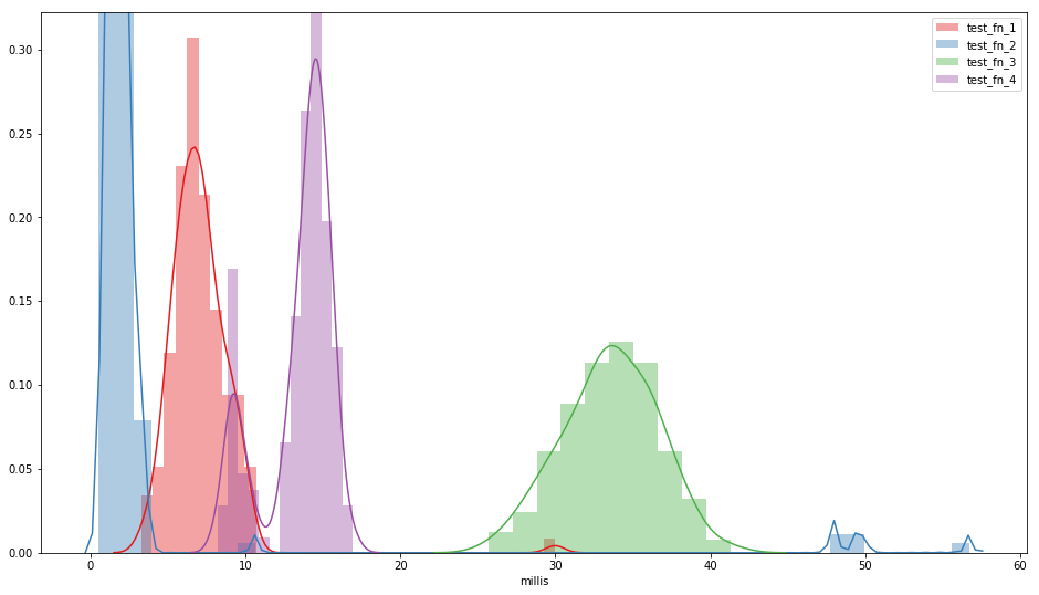
With these, and other charting libraries, you can do whatever you want with the data:
[8]:
from bokeh import palettes
import matplotlib.pyplot as plt
import seaborn as sns
%matplotlib inline

fig, ax = plt.subplots(figsize=(16, 9))
for col, color in zip(timings.columns, palettes.Set1[len(timings.columns)]):
    sns.distplot(timings[col], label=col, color=color, ax=ax,
#                  hist_kws=dict(cumulative=True),
#                  kde_kws=dict(cumulative=True)
                )
ax.set_xlabel('millis')
ax.legend()
timings.describe()
[8]:
| function | test_fn_1 | test_fn_2 | test_fn_3 | test_fn_4 |
|---|---|---|---|---|
| count | 158.000000 | 158.000000 | 158.000000 | 158.000000 |
| mean | 7.099615 | 3.423204 | 33.526883 | 13.455989 |
| std | 2.382655 | 8.588543 | 3.039051 | 2.193190 |
| min | 3.280499 | 0.548404 | 25.672770 | 8.190510 |
| 25% | 5.908776 | 1.335742 | 31.432720 | 12.909524 |
| 50% | 6.904165 | 1.840656 | 33.613588 | 14.226354 |
| 75% | 7.966824 | 2.353760 | 35.680228 | 14.863801 |
| max | 29.985672 | 56.681542 | 41.308623 | 16.934982 |
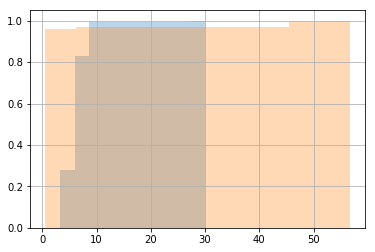
[9]:
import matplotlib.pyplot as plt
timings['test_fn_1'].hist(cumulative=True, normed=1, alpha=0.3)
timings['test_fn_2'].hist(cumulative=True, normed=1, alpha=0.3)
[9]:
<matplotlib.axes._subplots.AxesSubplot at 0x7f94c9fa8f28>
[10]:
import matplotlib.pyplot as plt
bt['test_fn_1'].hist(cumulative=True, normed=1, alpha=0.3)
bt['test_fn_2'].hist(cumulative=True, normed=1, alpha=0.3)
[10]:
<matplotlib.axes._subplots.AxesSubplot at 0x7f94c9d21a58>

[11]:
sns.pairplot(timings#, diag_kws={'cumulative': True}
            )
[11]:
<seaborn.axisgrid.PairGrid at 0x7f94c9ad46a0>

[12]:
import scipy.stats
bt = perfume.analyze.bucket_resample_timings(samples)
(scipy.stats.ks_2samp(timings['test_fn_1'], timings['test_fn_2']),
 scipy.stats.ks_2samp(bt['test_fn_1'], bt['test_fn_2']))
[12]:
(Ks_2sampResult(statistic=0.95569620253164556, pvalue=5.5872505324246181e-65),
 Ks_2sampResult(statistic=0.71199999999999997, pvalue=4.691029271698989e-223))